The LockRowIf function locks a row in a Wrap when a controlling cell is TRUE. After locking, the contents of a locked row cannot be modified.
You activate the function by inserting it into any cell in the row you want to lock. When the controlling cell returns TRUE, the LockRowIf function locks the row it is in. When a row is locked, no changes can be made to the fields in the row except for signature fields which have their own controlling cells and cannot be locked by LockRowIf.
There is a similar function that locks columns. There are also functions that hide rows or hide columns.
This example uses both the LockRowIf and LockColumnIf function. The user selects a day, which locks all but one of the day columns. The user then selects a measurement, which locks all but one of the measurement columns. As a result, it is only possible to change one number in the entire table. Locking parts of a complex table can dramatically increase data quality.
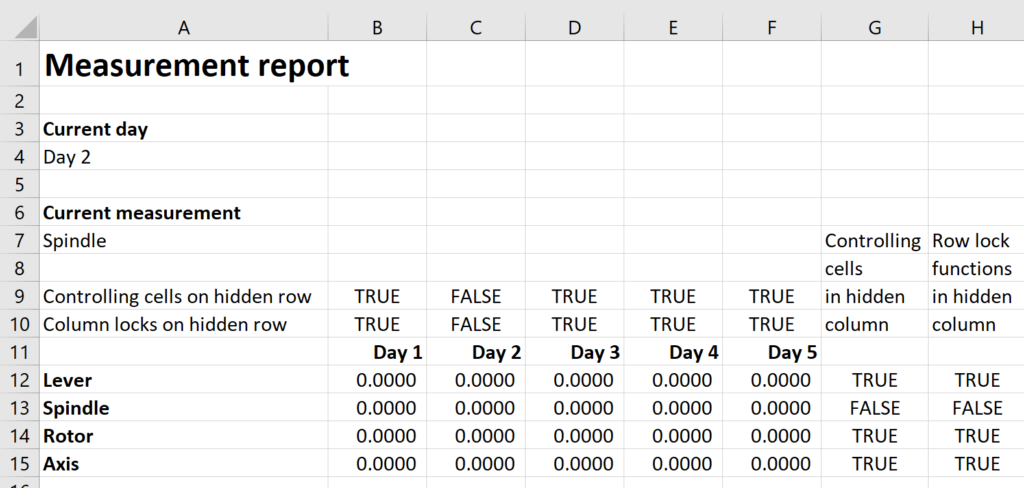
In the example above, you can see how access to the measurement data in A11:F15 is limited by the choices the user makes in the cur_day cell A4, and the cur_meas cell in A7.
Row 9 contains the controlling cells for columns. Each cell contains an expression similar to this formula in B9:
=cur_day<>B$11
This expression returns the result of the comparison. If cur_day in A4 is set to “Day 2” like in the screenshot above, it is not equal to B11 which contains “Day 1” so B9 returns TRUE. The formula has been copied to all the other four controlling cells for columns in C9:F9. Since cur_day in A4 can only have one value, only one of these controlling cells can be FALSE.
The same happens in G12:G15. Each controlling cell contains an expression similar to this formula in G12:
=cur_meas<>$A12
Again, the expression returns the result of the comparison. If cur_meas in A7 is set to “Spindle” like in the screenshot above, it is not equal to A12 which contains “Lever” so G12 returns TRUE. The formula has been copied to all the other controlling cells for rows in G13:G15. Since cur_meas in A7 can only have one value, only one of these controlling cells can be FALSE.
With all the controlling cells in place, we can now insert the function calls that will lock all the rows and columns that will not be affected by the new measurement.
The LockColumnIf function call in B10 looks like this:
=LockColumnIf(B9)
This will lock all of column B for modification if the controlling cell B9 is TRUE. The function also returns the current value of the controlling cell, which in the screenshot is TRUE, and so column B is locked. Similar function calls have been copied to C10:F10 and return the value of their respective controlling cells.
The LockRowIf function call in H12 looks like this:
=LockRowIf(G12)
This will lock all of row 12 for modification if the controlling cell G12 is TRUE. The function also returns the current value of the controlling cell, which in the screenshot is TRUE, and so row 12 is locked. Similar function calls have been copied to H13:H15 and return the value of their respective controlling cells.
You may want to hide both the LockRowIf and LockColumnIf functions and their controlling cells from the user. You can do this cell by cell with the Utility widget. In this example, we found it easier to hide all of rows 9-10 and all of columns G-H. We do this before conversion by right-clicking on them one at a time and then selecting Hide in the menu.
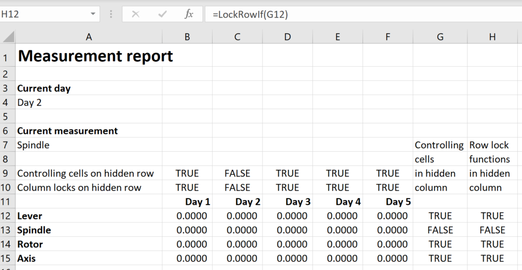
In this example, row 12 of the instance will be locked if the controlling cell in G12 returns TRUE.
This is what this LockRowIf function call will look like:
=LockRowIf(G12)
=LockRowIf(expression)
Locks the row that the HideRowIf function is placed in, if the expression is True.
The cell containing the LockRowIf function can be hidden or in a hidden column.
Specify the address or name of the controlling cell that returns TRUE when the row is to be locked. The controlling cell can be on a different row or worksheet than the row it is locking. The same controlling cell can be used by any number of LockRowIf functions on any number of sheets in the same workbook.
The controlling cell can be hidden, in a hidden row or column, and/or on a hidden sheet.
If the Wrap doesn’t already have a cell that you can use as the controlling cell, you can control the locking of the row with a condition directly in the LockRowIf function that either returns TRUE or FALSE. If the controlling cell G12 wasn’t already available in the Wrap in the example above, H12 could instead have evaluated the cur_meas setting to control the locking of row 12:
=LockRowIf(cur_meas<>$A12)
The controlling cell is an input cell and must be named. The cell with the LockRowIf widget does not have to be named, and naming it adds little value or readability.
Signature fields are unaffected by all locking mechanisms in ExcelWraps. This allows users with the required permissions to revoke a freeze signature, if necessary.
If you place the LockRowIf function in a merged cell, it counts as the lowest row number. Example: if A3:A6 are merged, and you place a LockRowIf function in the merged cell, it will lock row 3 only.