The HideColumnIf function hides a column in a Wrap when a controlling cell is TRUE. It works like when you hide rows with the Hide Rows/Sheets widget or the HideRowsIf function, but on columns instead of rows.
When a controlling cell returns TRUE, the HideColumnf function hides the column it is in. You activate the function by inserting it into any cell on the column you want to hide.
There is a similar function that hides unnecessary rows. There is also a function that locks rows and one that locks columns.
You wouldn’t ask a technician “how many problems were reported in the fifth carriage” if you knew the train only had three carriages. It is a common problem in Wraps and other web forms that some questions only need to be asked under certain conditions. Unless a question is relevant, it is often better to hide it from the user.
To create a Wrap that handles this situation automatically, you can begin by asking the respondent how many cars there are in the train. In the example below, their response will appear as a choice from the dropdown widget in cell B1, which is named car_count.
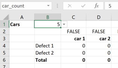
We will use column C and up to ask for information about defects in the corresponding carriage. We could create a separate controlling cell for each column but in this case, it is easier to use a condition directly in the HideColumnIf function call.
One of the advantages of the HideColumnIf function is that we can use Excel’s “fill right” feature, or copy/paste, to copy the HideColumnIf function call to each column. Let’s assume we insert a row of controlling cells as row 3 in the example above, and that the HideColumnIf function in C2 if expressed as =HideColumnIf(C3). When we copy/paste or fill this formula to the right, each HideColumnIf function will automatically reference its own controlling cell in the same column.
You may want to hide both the HideColumnIf function and its controlling cell from the user. You can do this with the Utility widget.
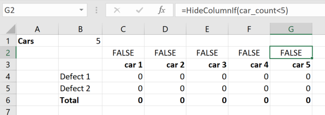
In this example, column G of the Wrap will be hidden if the car_count dropdown (in B1) is set to a value less than five.
This is what this HideColumnIf function call will look like:
=HideColumnIf(car_count<5)
=HideColumnIf(expression)
Hides the column that the HideColumnIf function is placed in if the expression is True.
The cell containing the HideColumnIf function can be hidden or in a hidden row.
Specify the address or name of the controlling cell that returns TRUE when the column is to be hidden. The controlling cell can be on a different column or worksheet than the column it is hiding. The same controlling cell can be used by any number of HideColumnIf functions on any number of sheets in the same workbook.
The controlling cell can be hidden, in a hidden row, and/or on a hidden sheet.
In the example above, we could have inserted a controlling cell in D3 with the formula
=car_count<2
However, this content would not fill down or copy/paste nicely, since you would have to manually change the number of cars for each column. To make it possible to use the same function for all the columns of the table, you could change it to
=car_count<COLUMN()-2
Since column D is the fourth column, this formula evaluates to the same condition as the one above, but it can now be copied unchanged to work also for all other columns in the spreadsheet. Perhaps a minor saving in this case with only five columns, but if your table includes many columns using a smarter formula can save time and reduce the risk of errors.
If the Wrap doesn’t already have a cell that you can use as the controlling cell, you can control the visibility of the column with a condition directly in the HideColumnIf function that either returns TRUE or FALSE like in the examples on this page.
The controlling cell is an input cell and must be named. The cell with the HideColumnIf widget does not have to be named, and naming it adds little value or readability.